using CairoMakie
using Downloads: download
using Format
using GregoryLoredo
using ZipStreams

A real life example of the Gregory & Loredo (1992) algorithm

This example of application of the GL92 algorithm is based on data published by Raywade et al.(2020). The Authors collected fast-radio bursts (FRBs) from the event FRB 121102 in order to identify a possible periodicity in the occurrence these events.

Of course, please be aware that the purpose of this exercise is showing a possible workflow for the package. This is not, and cannot be, a full and final scientific analysis of the considered data set!

Let's start!

Download the dataset

First of all, let's download the table with the events selected in this study. It is available as supplemental material at the site of the journal.

url = "https://oup.silverchair-cdn.com/oup/backfile/Content_public/Journal/mnras/495/4/10.1093_mnras_staa1237/1/staa1237_supplemental_files.zip?Expires=1766572517&Signature=adGzR1A9rTR87jcRkYgNoTttES089LNZfiERXSlFMe7PXiETHLtRVleSsvn8CXCEbRFdcPqTq30FYJkocKHpV11yZ395ny1j4zIvYP5uXRrZ47vqtyNw2lF0uHlQPtGL3PI0yFF0kjLEBNcVpfVs1igA753JRkIocmyrjdodoY03mBOVcvlv44riSBgEjLba5Jv-YgpfCnuq2J2NkDlh~N-GWM8QZu3frI4IhlMbbC69hai8Q9a4hc6OTHh1T7pqYcx-q78JT5tZBRWUUjeUU~cBl44OjZsALEFrYS4wyoQxVqunw9LX8ti-sTNCvn4QCb42cqWtw8KsqiXAikYR9Q__&Key-Pair-Id=APKAIE5G5CRDK6RD3PGA"

data = Vector{Float64}()

zipsource(download(url)) do source   # context management of sources with "do" syntax
    for f in source                  # iterate through files in an archive
        println(info(f).name)
        if info(f).name == "All_dets_paper.txt"
            open(info(f).name) do fdt
                l = readlines(fdt)
                for i in l
                    push!(data,parse(Float64,split(i)[2]))
                end
            end
        end
    end
end

Visualize the dataset

Let's plot an histogram showing the FRB detection epoch distribution in our dataset.

f = Figure()

ax = Axis(f[1,1],
    xlabel = "Time (MJD)",
    ylabel = "N",
    )

hist!(data)

f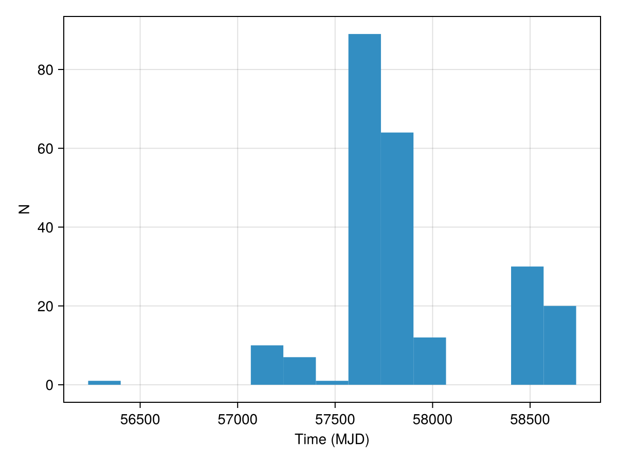

println("Data consists of ", length(data), " events.")

Data consists of 234 events.

We need to define a frequency range for the analysis. We can provide a range defined manually, or rely on an automatic generation baased on data length and range. We can have a linear or logarithmic spacing.

wr = FrequencyRange(data,logspacing=true)

whi = maximum(wr)
wlo = minimum(wr)

printfmtln("Minimum period: {:.1f} days, maximum period: {:.1f} days, number of periods: {:d}",2π/whi,2π/wlo,length(wr))

Minimum period: 10.7 days, maximum period: 250.3 days, number of periods: 117

Model parameter

The GL92 does not assume any specific light-curve shape, and describe the variability pattern as a box-shaped function. The maximum number of boxes is, in principle, only limited by the availabe computing power and data quality. For the dataset we are considering, we adopt a maximum number of boxes of 40.

mmax = 40;

Odd ratios

The first step is therefore to compute the odd ratios for each model (m from 2 to mmax) compared to the constant (no variability model, m=1).

omq = OddRatios(data,wr,mmax);

And plot the histogram of the obtained odd ratios:

PlotOddRatios(omq)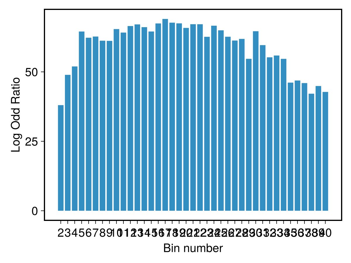

And derive some summary from the odd ratios distribution:

odrs = OddRatioSummary(omq)
printfmtln("Probability non-constant model: {:.2g} and best number of bins: {:d}", odrs.prob, odrs.maxm)

Probability non-constant model: 1.00 and best number of bins: 17

First of all, the probability for a non-constant model is extrenely high, and apart from the simplest caes with low m, the most probable models require m in the range approximately from 6 to 30. The highest probability is for m=17. Of course, pay attention to the logarithm scale of the plot.

Periodogram for the best m

Let's therefore compute and plot a periodogram for this choice of m:

mper = Periodogram(data,wr,odrs.maxm)
PlotPeriodogram(mper,wr)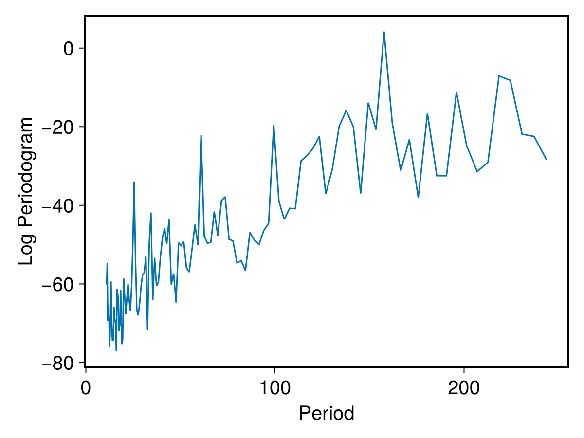

And let's derive some information from the periodogram data:

mpers = PeriodogramSummary(mper,wr)
printfmtln("Log maximum power: {:.2f}, angular frequency at maximum: {:.3f}, period: {:.2f} days",log10(mpers.maxpow),mpers.maxfreq,mpers.maxper)

Log maximum power: 4.20, angular frequency at maximum: 0.040, period: 157.69 days

The periodogram indeed shows a rather promiment peak at the period = 157.69 days. This is in reasonable agreement with what reported in Raywade et al.(2020), although based on different tools. It is also of interest comparing our periodogram with what reported in their paper, in Fig. 3.

Light-curve shape

Having derived the most probable frequency for a periodic behaviour, we can compute and plot the light-curve shape:

llpl = LightCurveShape(wr,odrs.maxm,data);
PlotLightCurve(llpl)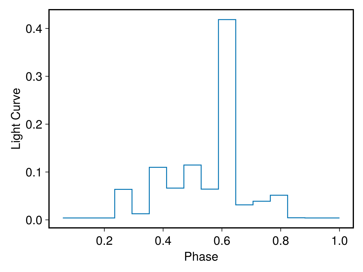

And, again, we can compare it with the analogous plot in Raywade et al.(2020), i.e., their Fig. 4. The two light-curves are very similar but now the phase is not assumed, it is just computed from the data.

Marginalized periodogram

Finally, rather than choosing the most probable m, it is also possible, and probably better justified, computing a periodogram marginalizing for m. Results are often very similar, specially if the most probable m stands clearly out the general distribution. But this is not always the case.

The marginalized periodogram can be computed and plotted with:

marmper = MarginalizedPeriodogram(data,wr,mmax)
PlotPeriodogram(marmper,wr)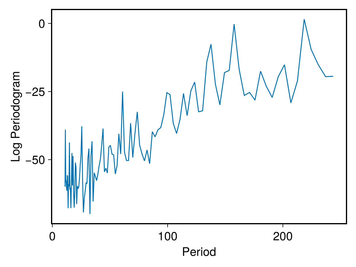

And let's see the usual summary:

marmpers = PeriodogramSummary(marmper,wr)
printfmtln("Log maximum power: {:.2f}, angular frequency at maximum: {:.3f}, period: {:.2f}",log10(marmpers.maxpow),marmpers.maxfreq,marmpers.maxper)

Log maximum power: 1.56, angular frequency at maximum: 0.029, period: 218.49 days

As a matter of fact, the peak at ~157 days is still there, but a new peak at ~218 days appears. Both peaks are now less promiment, possibly suggesting that the identified periodicity is not (basing upon the available data) very solid.